Integration in Mathematics: From Ancient Sums to Modern Calculus
In the realm of mathematics, an integral serves as the continuous analog of a sum. It is a powerful tool used to calculate areas, volumes, and their higher-dimensional generalizations. The process of computing these values, known as integration, stands as one of the two pillars of calculus, alongside differentiation. While initially developed to solve specific problems in physics and mathematics—such as determining displacement from velocity or finding the area under a curve—integration has since expanded into nearly every scientific field.
Key Facts
- Definite Integrals: Compute the signed area between a function's graph and the horizontal axis.
- Indefinite Integrals: Refer to the antiderivative of a function.
- Fundamental Theorem of Calculus: Establishes that differentiation and integration are inverse operations.
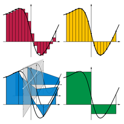
- Riemann vs. Lebesgue: Riemann integration uses thin vertical slabs, while Lebesgue integration provides a more general framework for a wider class of functions.
- Notation: The integral symbol & IntelliJ; was introduced by Gottfried Wilhelm Leibniz in 1675.
Foundational Concepts of Integration
A definite integral calculates the signed area of a region in a plane bounded by the graph of a function between two specific points on a real line. By convention, areas located above the horizontal axis are treated as positive, while those below are negative.
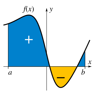
Conversely, when the limits of integration are omitted, the process refers to finding an antiderivative—a function whose derivative is the original function. These are known as indefinite integrals. The bridge between these two concepts is the fundamental theorem of calculus, which provides the method for computing definite integrals when the antiderivative is known.
The Process of Approximation
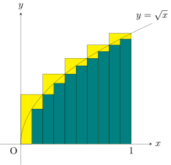
To understand how an integral reaches an exact value, one can use approximations. For example, to find the area under the function f(x) = √x from x = 0 to x = 1, the interval can be divided into several pieces. Using the right endpoint of each piece to determine the height of rectangles often results in an overestimate, while using the left endpoint often results in an underestimate. As the number of these pieces increases toward infinity, the sum converges to the exact area, which in this case is 2/3.
The Evolution of Integration
Pre-Calculus and Ancient Methods
Long before formal calculus, the ancient Greeks used the method of exhaustion. Developed by Eudoxus and Democritus around 370 BC and later refined by Archimedes, this technique involved breaking areas and volumes into an infinite number of known divisions. Archimedes applied this to calculate the area of circles, ellipses, and spirals, as well as the volume of spheres and paraboloids.
In the Middle East, Hasan Ibn al-Haytham (Alhazen) contributed significantly between 965 and 1040 AD by deriving formulas for the sum of fourth powers, which he used to calculate the volume of a paraboloid.
The Birth of Modern Calculus
The late 17th century marked a turning point when Isaac Newton and Gottfried Wilhelm Leibniz independently formulated the principles of integration. They conceptualized the area under a curve as an infinite sum of rectangles with infinitesimal width. Leibniz introduced the integral symbol & IntelliJ; in 1675, adapting it from the letter "s" for summa (Latin for sum).
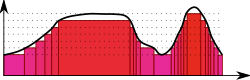
Later, Bernhard Riemann provided a rigorous definition based on a limiting procedure of thin vertical slabs. In the early 20th century, Henri Lebesgue further generalized this into the Lebesgue integral, allowing for the integration of a much broader class of functions.
Types of Integrals and Extensions
Integration extends far beyond simple areas under a curve. Depending on the domain and the goal, different types of integrals are employed:
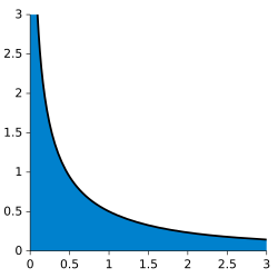
- Improper Integrals: Used when the intervals of the domain or range are unbounded.
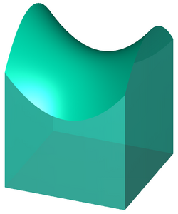
- Multiple Integrals: Such as double integrals, which compute the volume under a surface.
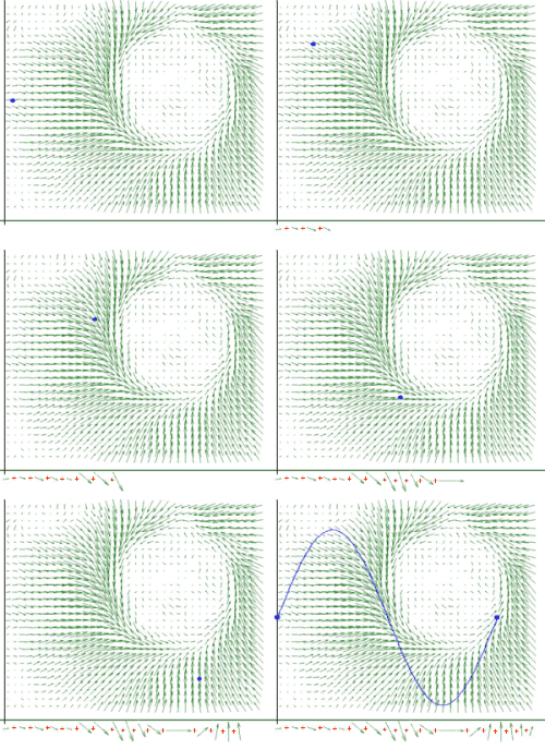
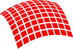
- Line and Surface Integrals: Line integrals sum elements along a curve, while surface integrals split a surface into small elements for calculation.
- Specialized Integrals: These include the Haar integral (for locally compact topological groups) and the Choquet integral (a subadditive or superadditive integral).
Summary of Integration Types
| Integral Type | Primary Purpose | Key Characteristic |
|---|---|---|
| Definite | Calculate signed area | Has specific upper and lower limits |
| Indefinite | Find the antiderivative | General form without limits |
| Improper | Handle unbounded regions | Infinite limits or discontinuities |
| Double | Calculate volume | Integrates over a 2D region |
| Line | Sum along a path | Evaluated along a specific curve |
Computational Methods
Integration can be performed through various analytical and numerical means. Symbolic integration uses rule-based systems, such as Rubi, which employs over 6,600 rules to match patterns and solve integrands. Another approach is the method of brackets, a generalization of Ramanujan's master theorem.
When an analytical solution is impossible, numerical quadrature is used. Common methods include:
- Romberg's Method: Uses trapezoid approximations and polynomial extrapolation to refine results.
- Gaussian Quadrature: Evaluates functions at the roots of orthogonal polynomials to achieve high precision.
- Rectangle and Trapezoidal Rules: Basic methods of approximating area via simple geometric shapes.
Frequently Asked Questions
What is the difference between a definite and an indefinite integral?
A definite integral results in a specific number representing the signed area between two limits. An indefinite integral results in a general function known as the antiderivative.
Who invented the integral symbol?
Gottfried Wilhelm Leibniz introduced the symbol & IntelliJ; in 1675, basing it on the Latin word summa.
How does the Fundamental Theorem of Calculus work?
It links differentiation and integration, stating that they are inverse operations. This allows the definite integral of a function to be calculated using its antiderivative.
What is a Lebesgue integral?
The Lebesgue integral is a generalization of the Riemann integral developed by Henri Lebesgue. It is more powerful because it can handle a wider variety of functions that are not Riemann-integrable.
What is numerical quadrature?
Numerical quadrature refers to a set of algorithms used to approximate the value of a definite integral when an exact symbolic solution is difficult or impossible to find.