SQUID Sensors: History, Design, and Superconducting Applications
A SQUID (Superconducting Quantum Interference Device) is an incredibly sensitive magnetometer used to measure extremely subtle magnetic fields. These devices rely on the principles of superconductivity and the Josephson effect—a phenomenon where an electric current flows across a non-superconducting barrier between two superconductors without any voltage applied.
The development of SQUIDs began in the early 1960s, following Brian Josephson's 1962 postulation of the Josephson effect and the subsequent creation of the first Josephson junction by John Rowell and Philip Anderson at Bell Labs in 1963. Since then, SQUIDs have evolved into two primary architectures: Direct Current (DC) and Radio Frequency (RF).
Key Facts
- Sensitivity: SQUIDs are among the most sensitive instruments for measuring magnetic flux.
- Core Component: They utilize Josephson junctions, which are thin barriers separating superconducting regions.
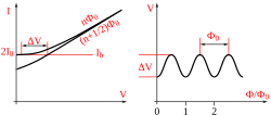
- Periodicity: The voltage response of a SQUID is periodic, with a period equal to one magnetic flux quantum (Φ₀).
- Cooling: Traditional SQUIDs require liquid helium, while high-temperature versions use liquid nitrogen.
- Types: DC SQUIDs are generally more sensitive, while RF SQUIDs are simpler and cheaper to produce.
DC SQUID: Design and Operation
Invented in 1964 by Robert Jaklevic, John J. Lambe, James Mercereau, and Arnold Silver at Ford Research Labs, the DC SQUID consists of two Josephson junctions connected in parallel within a superconducting loop. It operates based on the DC Josephson effect.
In a state with no external magnetic field, the input current (I) splits equally between the two branches. However, when an external magnetic field is applied, a screening current (Is) circulates the loop to cancel the external flux. This creates an additional Josephson phase proportional to the magnetic flux. This induced current adds to the input current in one branch and subtracts from it in the other. When the current in either branch exceeds the critical current (Ic)—the maximum current a junction can carry without resistance—a voltage appears across the junction.

As the external flux increases beyond half a magnetic flux quantum (Φ₀/2), the SQUID energetically prefers to increase the enclosed flux to a full integer multiple of Φ₀. This causes the screening current to reverse direction. Consequently, the current changes direction periodically every time the flux increases by a half-integer multiple of Φ₀.
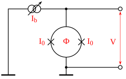
To eliminate hysteresis (a lag in the response), a shunt resistance (R) is often connected across the junction. In high-temperature superconductors based on copper oxide, the intrinsic resistance is usually sufficient. The relationship between voltage change (ΔV) and flux change (ΔΦ) can be expressed as:
ΔV = (R/L) ⋅ ΔΦ
Where L represents the self-inductance of the superconducting ring. In practical applications, the parameter λ = (Ic L / Φ₀) is typically around one.
RF SQUID: Design and Operation
The RF SQUID was invented in 1967 by the Ford Research team, including James Edward Zimmerman. Unlike the DC version, the RF SQUID uses only one Josephson junction and is based on the AC Josephson effect.
While less sensitive than DC SQUIDs, RF SQUIDs are cheaper and easier to manufacture in small quantities. They are widely used in biomagnetism to measure extremely small biological signals. An RF SQUID is inductively coupled to a resonant tank circuit; as the external magnetic field changes, the effective inductance of the tank circuit shifts, altering its resonant frequency. This change is measured as a periodic voltage across a load resistor.
Materials and Evolution
The choice of materials determines the operating temperature and sensitivity of the sensor:
| Material Type | Common Materials | Coolant | Characteristics |
|---|---|---|---|
| Traditional Low-Temp | Pure Niobium, Lead alloy (10% Gold/Indium) | Liquid Helium | Highest sensitivity; requires near absolute zero. |
| High-Temperature | YBCO | Liquid Nitrogen | Easier handling; lower sensitivity. |
| Nanoscale/Experimental | Carbon Nanotubes (CNT), Twisted Bilayer Graphene | Cryogenic (e.g., 1K) | Extremely small size; capable of counting spins. |
Traditional lead-based SQUIDs often use gold or indium alloys because pure lead is unstable during temperature cycling. In the late 1980s, high-temperature superconductors like YBCO allowed for the use of liquid nitrogen, which is more cost-effective. More recently, innovation has pushed into the nanoscale, with 2006 proof-of-concept CNT-SQUIDs (using single-walled carbon nanotubes) and 2022 developments using magic angle twisted bilayer graphene (MATBG).
Frequently Asked Questions
What is the main difference between a DC SQUID and an RF SQUID?
A DC SQUID uses two Josephson junctions in parallel and is generally more sensitive, whereas an RF SQUID uses a single Josephson junction, making it less sensitive but cheaper and easier to produce.
Why is liquid helium or nitrogen required for SQUIDs?
SQUIDs rely on superconductivity, a state where electrical resistance vanishes. This state only occurs when the materials are cooled below their specific critical temperature, which for traditional materials is only a few degrees above absolute zero.
What is a magnetic flux quantum (Φ₀)?
The magnetic flux quantum is the fundamental unit of magnetic flux that can pass through a superconducting loop. SQUID voltage responses are periodic based on this value.
What are SQUIDs used for in medicine?
RF SQUIDs, in particular, are frequently used in biomagnetism to detect the extremely weak magnetic fields produced by biological processes in the human body.
Can SQUIDs be made from carbon nanotubes?
Yes, proof-of-concept sensors were demonstrated in 2006 using an aluminium loop and a single-walled carbon nanotube Josephson junction, allowing for sensors only a few hundred nanometers in size.