Shepard's Method: Principles of Inverse Distance Weighting
In the realm of spatial analysis and data science, interpolation—the process of estimating unknown values based on known data points—is a fundamental tool. One of the most enduring techniques for this is Shepard's method, a form of Inverse Distance Weighting (IDW). Developed in the 1960s, this method provides a mathematically straightforward way to create a continuous surface from scattered data points.
The Origins of Shepard's Method
The method emerged from the Harvard Laboratory for Computer Graphics and Spatial Analysis starting in 1964. The laboratory, led by Howard Fisher, was a hub for scientists rethinking the foundations of what we now call Geographic Information Systems (GIS). Fisher had developed a computer mapping program called SYMAP, but he sought to improve its interpolation capabilities.
Donald Shepard, then a Harvard freshman, took on the challenge of overhauling SYMAP's interpolation. Influenced by the spatial analysis work of William Warntz and others at the lab, Shepard published his findings in 1968. He experimented with distance exponents, ultimately favoring a model similar to the gravity model (using an exponent of -2). Beyond basic weighting, Shepard's implementation was state-of-the-art for its time, incorporating the ability to handle both permeable and absolute barriers to interpolation.
How Shepard's Method Works
At its core, Shepard's method calculates an interpolated value as a weighted average of known sample points. The weight assigned to each known point is inversely proportional to its distance from the point being estimated.
The Mathematical Foundation
Given a set of sample points where each point has a known value, the interpolation function is defined as the sum of the weighted values divided by the sum of the weights. If the point being interpolated coincides exactly with a known point, the value of that known point is used.
The weighting function is defined as:
- Weight (w): The inverse of the distance (d) raised to a power parameter (p).
- Distance (d): The metric distance between the known point and the target point.
- Power Parameter (p): A positive real number that determines how quickly the influence of a point fades over distance.
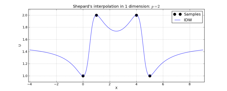
The Role of the Power Parameter (p)
The choice of the power parameter p significantly alters the resulting surface:
- High values of p: Give more influence to the closest points. As p becomes very large, the result resembles a Voronoi diagram (a mosaic of tiles), where each area has a nearly constant value based on the nearest point.
- Low values of p: Allow distant points to have a greater influence. In two-dimensional spaces, if p ≤ 2, the summed weight can diverge as the distance increases, meaning distant points may dominate the calculation.
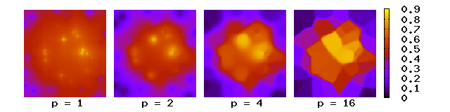
When selecting a value for p, practitioners consider the desired level of smoothing, the density of the sample distribution, and the maximum distance a sample should be allowed to influence its surroundings.
Advanced Variations and Extensions
Shepard's method is essentially a generalization of Lagrange approximation for multidimensional spaces. Over time, several modifications have been developed to increase efficiency and accuracy.
Modified Shepard's Method
To handle large-scale problems, a modified version calculates values using only the nearest neighbors within a specific radius (an R-sphere) rather than the entire dataset. By combining this approach with fast spatial search structures like kd-trees, the process becomes an efficient N log N interpolation method.
Additional Weighting Factors
To improve accuracy, multipliers can be added to the basic IDW function. These are typically validated through cross-validation. Examples include:
- Elevation Difference: Often used when interpolating wind speed.
- CUTHI: Applied when data is non-homogeneously distributed or clustered to reduce the "bullseye effect" (concentric circles around data points).
Key Facts
- Developer: Donald Shepard, an undergraduate at Harvard, published the method in 1968.
- Core Logic: Uses Inverse Distance Weighting (IDW) to estimate values.
- Power Parameter: The variable p controls the smoothing; higher values create a more "tiled" appearance.
- Dimensionality: The method is applicable to multidimensional spaces and generalizes Lagrange approximation.
- Efficiency: Modified versions using R-spheres and kd-trees optimize the method for large datasets.
| Parameter Value | Influence of Distant Points | Visual Result | Common Use Case |
|---|---|---|---|
| Low (p ≤ 2 in 2D) | High | Smooth, global influence | Broad trends |
| High (p > 2) | Low | Localized, "tiled" (Voronoi-like) | Local precision |
Frequently Asked Questions
What is the "bullseye effect" in IDW?
The bullseye effect occurs when the interpolation creates concentric circles of similar values around isolated sample points, making the map look like a series of targets rather than a natural surface.
How does the power parameter p affect the interpolation?
The power parameter determines the rate at which the influence of a known point decreases with distance. A higher p makes the interpolation more local, while a lower p allows distant points to influence the result more heavily.
Can Shepard's method be used for 3D data?
Yes, the method is designed for multidimensional spaces. Robert J. Renka even developed a modified version specifically for trivariate (3D) interpolation, available in the TOMS Library.
What is the difference between the basic and modified Shepard's method?
The basic method uses all available sample points for every calculation, which is computationally expensive. The modified method only considers points within a specific distance (R-sphere), significantly increasing speed for large datasets.
Why is the gravity model mentioned in the history of the method?
Donald Shepard used the gravity model's exponent of -2 as a theoretical basis for his experiments with the distance exponent, which helped define the standard behavior of IDW.