Adaptive Filters: Principles, Algorithms, and Applications

In the world of signal processing, an adaptive filter is a variable filter that automatically adjusts its own parameters to minimize the error between its output and a desired signal. Unlike fixed filters, adaptive filters can evolve in real-time, making them essential for environments where signal characteristics change over time.

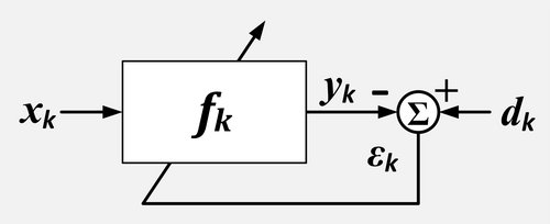
The core mechanism of a closed-loop adaptive filter is a feedback system. It takes a reference input and modifies it until it becomes a replica of the desired input. By minimizing the residual signal—the difference between the actual and desired output—the filter effectively isolates the target signal from interference.

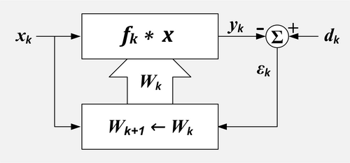
A block diagram of an adaptive filter with a separate block for the adaptation process. — Adaptive Filter. k = sample number, x = reference input, X = set of recent values of x, d = desired input, W = set of filter coefficients, ε = error output, f = filter impulse response, * = convolution, Σ = summation, upper box=linear filter, lower box=adaption algorithm

How Adaptive Filters Work

An adaptive filter operates using two primary input signals:

Primary Input (dk): This contains the desired signal combined with undesired interference.
Reference Input (xk): This contains signals that are correlated with the interference found in the primary input.

The filter is controlled by a vector of weights, denoted as Wk, which consists of L+1 coefficients. At each discrete sample time (k), the adaptation algorithm calculates a change in these weights (ΔWk). These adjustments are applied before the next sample (k+1) to refine the filter's performance.

A compact block diagram of an adaptive filter without a separate block for the adaptation process. — Adaptive Filter, compact representation. k = sample number, x = reference input, d = desired input, ε = error output, f = filter impulse response, Σ = summation, box=linear filter and adaption algorithm.

Signal Composition

To understand the mathematical process, we can break down the input signals into their components:

dk = gk + uk + vk (Desired signal + correlated interference + random noise)
xk = g'k + u'k + v'k (Correlated desired signal + correlated interference + random noise)

The filter produces an output (yk), and the resulting error signal (εk) is calculated as:

εk = dk − yk

Tapped Delay Line FIR Filters

A common implementation is the Finite Impulse Response (FIR) filter using a tapped delay line. In this structure, the impulse response is identical to the filter coefficients. The output is the summation of the weights multiplied by the delayed input samples:

yk = Σ (from l=0 to L) wlk x(k-l)

The Ideal Case

In an ideal scenario, there is no random noise (v = 0) and the reference input contains no part of the desired signal (g' = 0). Here, the reference input consists entirely of signals correlated with the interference (uk). When the filter converges, the output yk becomes the best mean square estimate of the interference. Subtracting this from the primary input leaves only the unchanged desired signal (gk).

Dealing with Signal Leakage

In real-world applications, the reference input often contains components of the desired signal (g' ≠ 0). While perfect cancellation is impossible here, the signal-to-interference ratio can still be improved. This relationship is governed by power inversion, where the output ratio is the reciprocal of the reference ratio:

ρout(z) = 1 / ρref(z)

For example, in a drive-thru window, a primary microphone picks up both the customer's voice and engine noise (1:1 ratio). A second reference microphone placed near the engine picks up mostly noise (50:1 ratio). An adaptive filter can use this reference to improve the primary signal's ratio to 50:1.

Adaptive Linear Combiners (ALC)

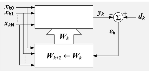
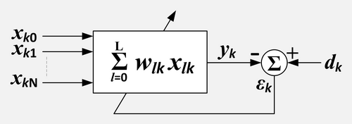
An Adaptive Linear Combiner is similar to an FIR filter but does not assume a temporal relationship between input values. Instead of delayed samples, the inputs (X) could be an array of pixels or outputs from multiple different delay lines. This makes ALCs ideal for adaptive beam forming in antenna or hydrophone arrays.

A block diagram of an adaptive linear combiner with a separate block for the adaptation process. — Adaptive linear combiner showing the combiner and the adaption process. k = sample number, n=input variable index, x = reference inputs, d = desired input, W = set of filter coefficients, ε = error output, Σ = summation, upper box=linear combiner, lower box=adaption algorithm.

A compact block diagram of an adaptive linear combiner without a separate block for the adaptation process. — Adaptive linear combiner, compact representation. k = sample number, n=input variable index, x = reference inputs, d = desired input, ε = error output, Σ = summation.

The Least Mean Squares (LMS) Algorithm

The Least Mean Squares (LMS) algorithm is a widely used method for updating filter weights. It makes small, incremental changes to each weight to reduce the error. The update formula for an FIR filter is:

wl,k+1 = wlk + 2μ εk xk-l

Here, μ is the convergence factor. The magnitude of the change depends on μ, the input value, and the current error. If the error is zero, no change occurs.

Convergence and Stability

The choice of μ is critical for performance:

Too large: The algorithm may fail to converge.
Too small: Convergence is slow, and the filter may not track changing conditions.
Balanced: The filter reaches steady state quickly but may overshoot the optimum weight.

To ensure convergence, μ must typically fall within the range: 0 < μ < 1/σ², where σ² is the total input power. This leads to the normalized LMS algorithm, which simplifies the convergence criteria to 0 < μσ < 1.

Nonlinear Adaptive Filters

Linear models have limitations that nonlinear filters aim to overcome. Various approaches are used to handle complex data:

Volterra and Kernel LMS: These replace standard data samples with nonlinear algebraic expressions.
Spline Adaptive Filters: These use a cascade of a linear dynamic block and a static nonlinearity approximated by splines.
Urysohn Adaptive Filters: These replace linear terms with piecewise linear functions identified from data samples.
Neural Networks: Often categorized as nonlinear adaptive filters due to their ability to model complex mappings.

Key Facts

Primary Goal: Minimize the error (ε) between the filter output and a desired signal.
Common Types: Least Mean Squares (LMS) and Recursive Least Squares (RLS).
LMS Update: Weights are adjusted based on the convergence factor (μ), the error, and the input signal.
Power Inversion: In cases of signal leakage, the output signal-to-interference ratio is the reciprocal of the reference ratio.
ALC Use Case: Adaptive Linear Combiners are frequently used in beam forming for antennas and hydrophones.

Component	Symbol	Description
Primary Input	dk	Desired signal + interference
Reference Input	xk	Signal correlated with interference
Filter Weights	Wk	Coefficients controlling the filter output
Error Signal	εk	Difference between desired and actual output
Convergence Factor	μ	Controls speed and stability of adaptation

Frequently Asked Questions

What is the difference between an FIR filter and an Adaptive Linear Combiner?

An FIR filter specifically uses a tapped delay line where inputs are sequential samples of the same signal. An Adaptive Linear Combiner (ALC) does not assume any relationship between its inputs, allowing it to process diverse data like pixel arrays or multiple different signal sources.

How does the convergence factor (μ) affect the LMS algorithm?

The convergence factor determines the trade-off between speed and stability. A high μ allows the filter to adapt quickly but risks instability or overshooting the optimum weights. A low μ ensures stability but results in slower convergence and poor tracking of dynamic signals.

What happens if the reference input contains the desired signal?

This is known as signal leakage. In this case, the filter cannot perfectly cancel the interference because it will also attempt to cancel the desired signal. However, the overall signal-to-interference ratio can still be improved via power inversion.

When should nonlinear adaptive filters be used?

Nonlinear filters, such as Volterra or Urysohn filters, should be used when the relationship between the input and the desired output cannot be accurately modeled by a linear combination, allowing for the processing of more complex, non-linear signal distortions.