Sea level: The Science of Earth's Vertical Datum
When we talk about the height of a mountain or the depth of a valley, we almost always reference "sea level." But what exactly is sea level? In scientific terms, this is known as Mean Sea Level (MSL)—the average surface level of Earth's coastal bodies of water. MSL serves as a vertical datum, which is a standardized reference point used in cartography, marine navigation, and aviation to measure elevation and altitude.
While it may seem like a simple flat line, MSL is a complex measurement influenced by gravity, planetary shape, and climate. Understanding how it is measured and why it changes is critical for everything from flying aircraft to predicting the future of our coastal cities.
The Geometry of the Ocean: Spheroids and Geoids
Earth is not a perfect sphere; it is a flattened spheroid, meaning it bulges at the center. Its radius at the equator is 6,378.137 km (3,963.191 mi), while at the poles, it shrinks to 6,356.752 km (3,949.903 mi), with a global average of 6,371.001 km (3,958.756 mi).
Because of this shape and local variations in gravity, scientists use a model called the geoid. The geoid is an equipotential surface of Earth's gravitational field—essentially a representation of what the ocean surface would look like if only gravity and rotation were at play, without the influence of tides or currents. The geoid is not uniform; for example, there is a significant depression in the Indian Ocean where the surface dips as much as 106 m (348 ft) below the global mean.
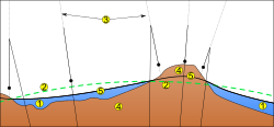
In practice, there is often a difference between the geoid and the actual measured sea level. A 2026 study revealed an "interdisciplinary blind spot," finding that 90% of published work used geoid models that underestimated sea levels by an average of 24–27 cm. In some cases, the discrepancy reached 550–760 cm. This underestimation is significant: for every 1 meter of sea level rise, 37% more coastal areas—affecting up to 132 million people—will fall below sea level than previously estimated.
How Mean Sea Level is Measured
Determining a precise MSL is challenging because the ocean is in constant motion. Factors such as wind, atmospheric pressure, salinity, temperature, and tsunamis cause instantaneous sea levels to fluctuate.
Tide Gauges and Local Datums
To find a stable average, scientists use still-water level (SWL), which averages out wind waves. MSL is then calculated by averaging the SWL over a long period—sometimes a full 19-year Metonic lunar cycle—at a specific reference location using a tide gauge.
Because different regions have different needs, many countries use their own local datums. For example, the UK's ordnance datum is based on measurements from Newlyn in Cornwall (1915–1921), while France uses the Marégraphe in Marseille, which has provided continuous data since 1883. Other references include the Kronstadt Sea-Gauge in Russia and the Amsterdam Peil in the Netherlands.
Satellite Altimetry
Since 1992, satellite altimeters have provided a more global perspective. Starting with the TOPEX/Poseidon mission (a joint effort by NASA and CNES), followed by Jason-1 and Jason-2, satellites can now measure the ocean surface with extreme precision from space.
Height Above Mean Sea Level (AMSL)
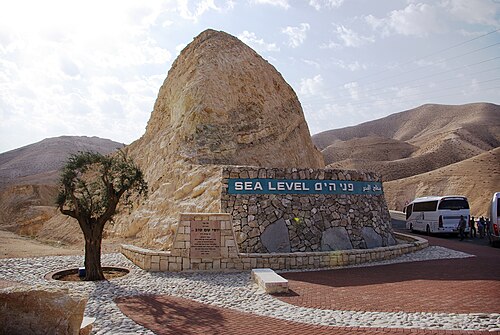
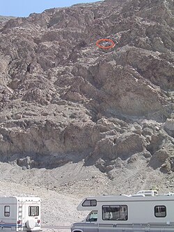
The term Height Above Mean Sea Level (AMSL) refers to the elevation of a point on land or the altitude of an object in the air relative to the MSL datum. On topographic maps, this is shown via contour lines. While most summits have a positive AMSL, some locations, such as Death Valley in California, have a negative AMSL because they sit below the reference sea level.
MSL in Aviation
In aviation, MSL is vital for safety. Pilots use altimeters set to a specific barometric pressure, known as QNH, which represents the pressure at MSL in their current region. This allows them to estimate their height above the ground by subtracting the known terrain altitude from their altimeter reading. Once aircraft reach a certain "transition altitude," they switch to the International Standard Atmosphere (ISA) pressure of 1013.25 hPa (29.92 inHg) to maintain consistent flight levels.
The Dynamics of Sea Level Change
Sea level is not static. Changes can be categorized by their cause and scale. The following table summarizes the primary types of sea level fluctuations:
| Term | Scope | Primary Cause |
|---|---|---|
| Relative | Local | Combination of water volume change and land movement. |
| Eustatic | Global | Changes in total water volume (e.g., melting ice caps) or ocean basin size. |
| Steric | Global | Thermal expansion of water as it warms or changes in salinity. |
| Isostatic | Local | Vertical movement of land (e.g., post-glacial rebound or tectonic shifts). |
For instance, isostatic post-glacial rebound occurs when land rises after the heavy weight of ice sheets from the last ice age melts away. Conversely, land can sink due to the weight of cooling volcanoes or the withdrawal of groundwater, leading to a relative rise in sea level.
Recent Trends and Future Projections
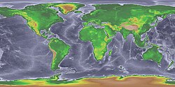
Global sea levels have been rising since the end of the Last Glacial Maximum approximately 20,000 years ago.
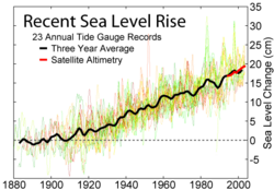
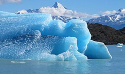
Between 1901 and 2018, the average sea level rose by 15–25 cm. The rate of increase has accelerated significantly: from 2.3 mm per year since the 1970s to 4.62 mm per year between 2013 and 2022. This acceleration is primarily driven by human-induced climate change.
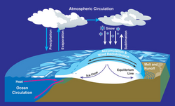
Between 1993 and 2018, the rise was split almost evenly between two factors: melting ice sheets and glaciers (44%) and the thermal expansion of warming water (42%).
Future Outlook and Human Impact
Because sea level rise lags behind temperature changes by decades, acceleration is expected to continue through 2050. Projections for the year 2100 vary based on greenhouse gas emissions:
- Low emissions: A rise of 30 cm to 1.0 m.
- High emissions: A rise of 50 cm to 1.9 m.
- Long-term (2,000 years): A rise of 2–3 m if warming stays at 1.5°C, but potentially 19–22 m if warming peaks at 5°C.
The consequences are severe, ranging from the loss of mangrove ecosystems and reduced crop yields due to saltwater intrusion to the total displacement of populations on low-lying Caribbean and Pacific atolls. While wealthier nations may implement "hard" adaptations like seawalls or "soft" approaches like beach nourishment, socially and economically vulnerable communities often face the highest risks with the fewest resources for relocation or protection.