Probability Theory: Foundations, History, and Mathematical Applications
At its core, probability is the numerical description of how likely an event is to occur. Expressed as a value between 0 and 1—or as a percentage from 0% to 100%—probability provides a mathematical framework for quantifying uncertainty. For instance, tossing a fair coin results in two equally likely outcomes: heads or tails. Because no other results are possible, the probability for either is 1/2, 0.5, or 50%.
This field has evolved into a rigorous axiomatic mathematical formalization known as probability theory. Today, it is indispensable across diverse disciplines, including statistics, finance, artificial intelligence, machine learning, computer science, game theory, and philosophy. Beyond simple predictions, it is used to describe the underlying mechanics of complex systems and draw inferences about the expected frequency of events.
Key Facts
- Probability Range: Always falls between 0 (impossible/almost never) and 1 (certain/almost certainly).
- Theoretical vs. Empirical: Theoretical probability is based on well-defined random experiments, while empirical probability is derived from real-world observations.
- Sample Space: The complete set of all possible results of an experiment.
- Normal Distribution: Also known as the Gauss law, it describes the frequency of errors as an exponential function of the square of the error.
- Bayes' Rule: A fundamental formula relating the conditional and marginal probabilities of random variables.
Interpretations of Probability
In a theoretical setting, probability is calculated by dividing the number of desired outcomes by the total number of all possible outcomes. For example, if you toss a coin twice, there are four possible outcomes: head-head, head-tail, tail-head, and tail-tail. The probability of getting "head-head" is 1 out of 4 (25%), while the probability of getting at least one head is 3 out of 4 (75%).
While theoretical probability works for idealized experiments, practical applications often split into two major competing interpretations regarding the fundamental nature of probability.
The Evolution of Probability Theory
Early Foundations
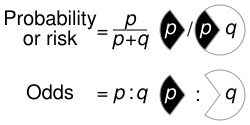
The formalization of probability began in the 16th century with the Italian polymath Gerolamo Cardano, who defined odds as the ratio of favorable to unfavorable outcomes.

The field advanced significantly in 1654 through the correspondence between Pierre de Fermat and Blaise Pascal. Shortly after, in 1657, Christiaan Huygens published one of the first scientific treatments of the subject.

By the early 18th century, Jakob Bernoulli's Ars Conjectandi (1713) and Abraham de Moivre's Doctrine of Chances (1718) established probability as a formal branch of mathematics.
The Theory of Errors and the Normal Distribution
The study of observational errors began with Roger Cotes and was furthered by Thomas Simpson in 1755, who introduced the concept of a probability curve. Pierre-Simon Laplace later proposed two laws of error. His second law (1778) stated that error frequency is an exponential function of the square of the error—a concept now known as the normal distribution or Gauss law.
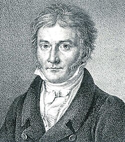
Further refinements came from Adrien-Marie Legendre, who developed the method of least squares in 1805, and Robert Adrain, who deduced the law of facility of error in 1808. Carl Friedrich Gauss provided the first European proof of this law in 1809.
Modern Developments
The 19th and 20th centuries saw the theory expand through the work of Karl Pearson, George Boole, and Augustus De Morgan. In 1906, Andrey Markov introduced Markov chains, which are critical to the study of stochastic processes (systems that evolve randomly over time). Finally, in 1931, Andrey Kolmogorov developed the modern theory of probability based on measure theory.
Mathematical Treatment of Events
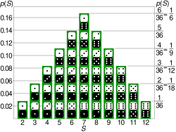
To analyze probability mathematically, we define a sample space (denoted as Ω), which is the collection of all possible results of an experiment. An event is a subset of this sample space. For example, when rolling a six-sided die, the sample space is {1, 2, 3, 4, 5, 6}. An event could be "rolling an odd number," represented by the subset {1, 3, 5}.
Complementary and Mutually Exclusive Events
The complement of an event A (denoted as not A) is the event that A does not occur. Its probability is calculated as P(not A) = 1 − P(A). For example, the probability of not rolling a six is 1 − 1/6 = 5/6.
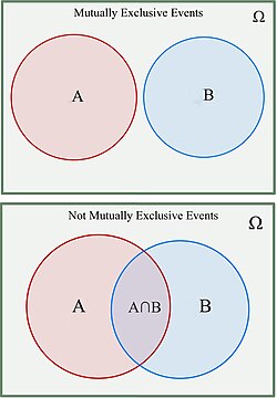
Mutually exclusive events are those that cannot happen at the same time. For instance, rolling a 1 and rolling a 2 on a single die are mutually exclusive. The probability of either occurring is simply the sum of their individual probabilities.
Non-Mutually Exclusive and Conditional Probability
If events are not mutually exclusive, they may overlap. When calculating the probability of either event occurring, the overlap must be subtracted to avoid double-counting. For example, when drawing a card, the probability of getting a heart or a face card is the sum of hearts (13) and face cards (12), minus the cards that are both (3).
Conditional probability occurs when the probability of an event depends on a previous outcome. In a bag with 2 red and 2 blue balls, the initial probability of picking a red ball is 2/4. If a red ball is removed, the probability of picking another red ball drops to 1/3.
Inverse Probability and Bayes' Rule
Bayes' rule relates the odds of an event before (prior) and after (posterior) conditioning on another event. It is often expressed as: posterior is proportional to prior times likelihood. This rule is fundamental for updating probabilities as new evidence becomes available.
Probability Summary Table
| Concept | Description | Key Formula/Value |
|---|---|---|
| Probability Range | The scale of likelihood for any event | 0 to 1 (or 0% to 100%) |
| Complementary Event | The probability of an event NOT occurring | P(not A) = 1 − P(A) |
| Mutually Exclusive | Events that cannot occur simultaneously | P(A or B) = P(A) + P(B) |
| Non-Mutually Exclusive | Events that can overlap | P(A or B) = P(A) + P(B) − P(A and B) |
| Theoretical Probability | Based on possible outcomes in a controlled setting | Desired Outcomes / Total Outcomes |
Frequently Asked Questions
What is the difference between theoretical and empirical probability?
Theoretical probability is based on the known possible outcomes of a well-defined experiment (like a coin flip), whereas empirical probability is based on the actual results of real-world experiments and observations.
What does a probability of 0 or 1 actually mean?
In finite sample spaces, 0 means impossible and 1 means certain. However, in infinite sample spaces, a probability of 0 indicates an event "almost never" takes place, and 1 indicates it "almost certainly" takes place, meaning the event is still possible even if its probability is 0.
What is a Markov chain?
Introduced by Andrey Markov in 1906, a Markov chain is a mathematical system that transitions from one state to another based on certain probabilistic rules, where the next state depends only on the current state and not on the sequence of events that preceded it.
How does Bayes' rule work in simple terms?
Bayes' rule allows you to update the probability of a hypothesis as more evidence or information becomes available. It calculates the posterior probability by combining the prior probability with the likelihood of the evidence.
What is the normal distribution?
The normal distribution, or Gauss law, is a probability distribution that describes how values of a variable are distributed. It is characterized by a symmetric, bell-shaped curve where most observations cluster around the central peak.