Multipath Mathematical Modeling in Wireless Communications
In wireless communication, signals rarely travel in a single, straight line from transmitter to receiver. Instead, they encounter obstacles that cause the signal to reflect, diffract, and scatter, creating multiple paths for the electromagnetic energy to reach its destination. This phenomenon, known as multipath propagation, can be analyzed using the mathematical framework of linear systems to understand how it affects signal integrity.
The Impulse Response Method
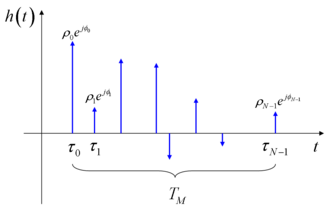
To model a multipath environment, engineers often use the impulse response method. Imagine transmitting a single, ideal Dirac pulse—an infinitely short pulse of electromagnetic power—at time zero. In a perfect vacuum with a single path, the receiver would see one pulse. However, in a multipath environment, the receiver detects multiple pulses arriving at different times.
These timing differences occur because electromagnetic signals travel at the speed of light; since each path has a different geometrical length, the travel time varies. For instance, in free space, light takes approximately 3 μs to travel a 1 km span.
The received signal, which serves as the impulse response function h(t), is expressed as the sum of these arriving pulses:
y(t) = h(t) = ∑ ρₙ eʲᶠⁿ δ(t − τₙ)
- N: The total number of received impulses (representing the number of paths).
- τₙ: The time delay of the n-th impulse.
- ρₙ eʲᶠⁿ: The complex amplitude, encompassing both the magnitude and the phase of the received pulse.
Time-Varying Conditions
In real-world scenarios, the geometrical conditions of reflections are rarely static. When the environment changes—such as when a transmitter or receiver moves—the impulse response becomes time-varying. In these cases, the time delay (τₙ), magnitude (ρₙ), and phase (ϕₙ) are all functions of time t.
Measuring Multipath Severity: Delay Spread
A critical metric used to quantify the severity of multipath conditions is the delay spread (Tₘ). This is defined as the time interval between the arrival of the first pulse and the last pulse:
Tₘ = τₙ₋₁ − τ₀
In practical measurements, the "last impulse" is typically defined as the point at which a specific percentage of the total transmitted power (e.g., 99%) has been received, after accounting for atmospheric and propagation losses.
The Channel Transfer Function
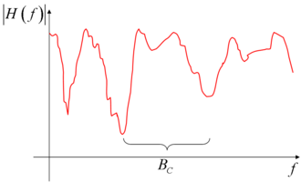
For linear, time-invariant systems, the multipath phenomenon can also be characterized in the frequency domain using the channel transfer function H(f). This function is the continuous-time Fourier transform of the impulse response h(t).
Because the Fourier transform of a Dirac pulse is a complex exponential function, the transfer function is represented as the sum of these exponentials across all paths. Visually, this results in a frequency response characterized by a series of peaks and valleys, the latter of which are often referred to as notches.
Coherence Bandwidth
The distance in Hz between these consecutive peaks or valleys is inversely proportional to the multipath time. This leads to the concept of coherence bandwidth (B꜀), which is approximately the reciprocal of the delay spread:
B꜀ ≈ 1 / Tₘ
For example, if a system has a multipath time of 3 μs (equivalent to an additional 1 km of travel for the final impulse), the resulting coherence bandwidth is approximately 330 kHz.
Key Facts
- Multipath Propagation: Occurs when signals take multiple geometrical paths to reach a receiver, causing time delays.
- Speed of Light: In free space, signals travel 1 km in approximately 3 μs.
- Delay Spread (Tₘ): The time difference between the first and last significant received impulses.
- Coherence Bandwidth (B꜀): The frequency range over which the channel is considered constant, calculated as 1/Tₘ.
- Channel Notches: Valleys in the transfer function caused by the interference of multipath signals.
| Parameter | Symbol | Definition/Relationship | Unit |
|---|---|---|---|
| Impulse Response | h(t) | Sum of delayed Dirac pulses | Time domain |
| Delay Spread | Tₘ | τₙ₋₁ − τ₀ | Seconds (s) |
| Transfer Function | H(f) | Fourier transform of h(t) | Frequency domain |
| Coherence Bandwidth | B꜀ | ≈ 1 / Tₘ | Hertz (Hz) |
Frequently Asked Questions
What is a Dirac pulse in the context of multipath modeling?
A Dirac pulse is an ideal, infinitely short pulse of electromagnetic power used as a mathematical tool to study how a linear system (like a wireless channel) responds over time.
How does the speed of light affect signal delay?
Since electromagnetic signals travel at the speed of light, any difference in the physical length of the paths they take results in different arrival times. For every 1 km of additional path length, a delay of roughly 3 μs is introduced.
What is the difference between delay spread and coherence bandwidth?
Delay spread is a time-domain measurement of the gap between the first and last arriving signals. Coherence bandwidth is the frequency-domain equivalent, representing the range of frequencies that experience similar fading.
What are "notches" in a channel transfer function?
Notches are the "valleys" or deep dips in the frequency response of a channel. They occur where multipath signals interfere destructively, significantly reducing the signal strength at those specific frequencies.
Why is the impulse response sometimes time-varying?
The impulse response becomes time-varying when the physical environment changes, such as when the transmitter, receiver, or surrounding reflecting objects move, altering the path lengths and reflection conditions.