Least Squares Regression: Principles, History, and Applications

In the realm of regression analysis, least squares is a fundamental method used to determine the best-fit model for a set of data. It achieves this by minimizing the sum of the squared residuals—the differences between the observed values and the values predicted by the mathematical model. By reducing these discrepancies, researchers can identify the most accurate relationship between variables.

Key Facts

Core Objective: Minimizes the sum of squared residuals to find the optimal model parameters.
Two Main Types: Linear (closed-form solution) and Nonlinear (solved via iterative refinement).
Historical Giants: Developed and refined by mathematicians including Legendre, Gauss, and Laplace.
Optimal Conditions: Under the Gauss-Markov theorem, it is the best linear unbiased estimator when errors are uncorrelated and have equal variance.
Broad Utility: Essential in astronomy, geodesy, and various scientific fields for predicting trends and fitting curves.

The Evolution of Least Squares

The method of least squares was not a single discovery but the culmination of 18th-century mathematical advances. Early concepts appeared in Isaac Newton's unpublished work in 1671 and 1700, suggesting that aggregating observations decreases error. Roger Cotes formally expressed these ideas in 1722.

Throughout the mid-to-late 1700s, the "method of averages" was employed by Newton, Tobias Mayer, and Pierre-Simon Laplace to study celestial motions. Simultaneously, the "method of least absolute deviation" was used by Roger Joseph Boscovich and Laplace to analyze the shape of the Earth.

The first concise exposition of the method was published by Adrien-Marie Legendre in 1805, describing it as an algebraic procedure for fitting linear equations. Shortly after, in 1809, Carl Friedrich Gauss published his work on calculating celestial orbits, claiming he had used the method since 1795.

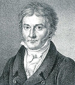
Gauss significantly advanced the field by linking least squares to the normal distribution (the bell curve) and probability theory. His method proved its power when he successfully predicted the location of the asteroid Ceres after it had been lost from view, using data that other astronomers found insufficient.

How the Method Works

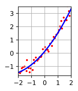
The goal of least squares is to adjust the parameters of a model function to best fit a data set. For a set of $n$ points, the fit is measured by the residual: the difference between the observed dependent variable and the model's predicted value.

The method finds the optimal parameters by minimizing the sum of these squared residuals. In its simplest form, this result is the arithmetic mean of the input data. For a two-dimensional straight line, the model identifies the optimal slope and y-intercept.

The result of fitting a set of data points with a quadratic function

Analyzing Residuals

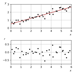
Residual plots are used to determine if a chosen model is appropriate. If the residuals show random fluctuations around zero, a linear model is typically sufficient.

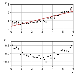
The values and residuals are plotted against corresponding values. The random fluctuations about indicate a linear model is appropriate.

However, if the residuals exhibit a parabolic shape, it indicates that a nonlinear or parabolic model would be more accurate.

The values and residuals are plotted against the corresponding values. The parabolic shape of the fluctuations about indicates a parabolic model would be more appropriate.

Linear vs. Nonlinear Least Squares

Least squares problems are categorized based on whether the model functions are linear in all unknowns.

Linear Least Squares (LLSQ)

A model is linear if it consists of a linear combination of parameters. LLSQ problems have a closed-form solution, meaning they can be solved directly using matrix algebra. The solution in LLSQ is unique.

Conic fitting a set of points using least-squares approximation

Nonlinear Least Squares (NLLSQ)

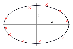
In NLLSQ, parameters appear as functions (e.g., exponents). These problems are typically solved through iterative refinement, such as the Gauss-Newton algorithm, where the system is approximated by a linear one at each step. Unlike linear models, NLLSQ may have multiple minima.

Limitations and Advanced Variations

Standard least squares assumes that errors occur only in the dependent variable. If errors in the independent variable are non-negligible, total least squares may be used to balance different error sources.

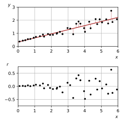
Another challenge is heteroscedasticity, where the variance of errors is not constant, often appearing as a "fanning out" effect in data plots.

"Fanning out" effect of heteroscedasticity

Regularization and Lasso

To prevent overfitting, regularization techniques are used. The Lasso method (Least Absolute Shrinkage and Selection Operator) adds a constraint based on the L1-norm of the parameter vector. This is equivalent to applying a zero-mean Laplace prior distribution in a Bayesian context.

Summary of Least Squares Types

Feature	Linear Least Squares (LLSQ)	Nonlinear Least Squares (NLLSQ)	Lasso Regression
Parameter Form	Linear combination	Functional/Nonlinear	Linear with L1 penalty
Solution Method	Closed-form (Matrix)	Iterative refinement	Convex optimization
Uniqueness	Unique solution	Potential multiple minima	Promotes sparsity
Primary Use	Simple trend fitting	Complex physical laws	Feature selection/Regularization

Frequently Asked Questions

What is a residual in least squares?

A residual is the vertical distance between an observed data point and the value predicted by the model. It represents the error for a single observation.

What is the Gauss-Markov theorem?

The Gauss-Markov theorem states that in a linear model where errors have a mean of zero, are uncorrelated, and have equal variances, the least-squares estimator is the best linear unbiased estimator (BLUE), meaning it has the minimum variance.

When should I use Nonlinear Least Squares instead of Linear?

You should use NLLSQ when the relationship between the independent and dependent variables cannot be expressed as a linear combination of parameters, such as in exponential growth or complex orbital mechanics.

How does the Lasso method differ from standard least squares?

While standard least squares simply minimizes the sum of squared residuals, Lasso adds a penalty based on the absolute size of the coefficients. This can force some coefficients to zero, effectively performing feature selection.

What happens if the residuals are not randomly distributed?

If residuals show a pattern (like a curve), it suggests that the model is misspecified. For example, a parabolic pattern in residuals indicates that a linear model is inappropriate and a higher-order polynomial should be used.