Computational Fluid Dynamics: Methodology, Discretization, and Turbulence Modeling
Computational Fluid Dynamics (CFD) is a powerful branch of fluid mechanics that uses numerical analysis and data structures to analyze and solve problems involving fluid flows. By transforming the complex partial differential equations that govern fluid motion into a format that computers can process, engineers and scientists can simulate everything from the aerodynamics of a supercar to the flow of blood through a human artery.
The CFD Workflow
Regardless of the specific numerical approach, most CFD simulations follow a standardized three-step procedure to ensure accuracy and consistency.
- Preprocessing: In this phase, the physical modeling is defined. This includes selecting the governing equations—such as fluid motion, enthalpy, radiation, and species conservation. Engineers also define boundary conditions, which specify fluid behavior and properties at the edges of the domain. For transient (time-dependent) problems, initial conditions are established here.
- Simulation: The computer solves the defined equations iteratively. Depending on the goal, the simulation may be run as a steady-state (constant over time) or transient analysis.
- Post-processing: The resulting data is analyzed and visualized to derive meaningful physical insights.
Discretization Methods
Discretization is the process of dividing a continuous fluid domain into a discrete set of points or volumes so that the governing equations can be solved numerically.
Finite Volume Method (FVM)
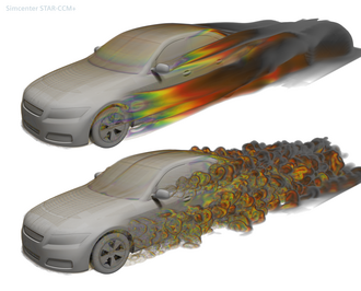
The Finite Volume Method is widely used in commercial CFD codes due to its efficiency in memory usage and solution speed. It is particularly effective for large-scale problems, high Reynolds number turbulent flows, and source-term dominated flows like combustion. FVM recasts governing equations into a conservative form and solves them over discrete control volumes, ensuring that fluxes are conserved across the volume.
Finite Element Method (FEM)
While primarily used in structural analysis for solids, FEM is also applicable to fluids. It is generally more stable than FVM and provides higher accuracy for smooth problems and complex geometries. However, it requires careful formulation to ensure conservation and typically demands more memory and longer computation times.
Finite Difference Method (FDM)
The Finite Difference Method is a fundamental approach that approximates derivatives using difference equations, solving for conserved variables and fluxes across the x, y, and z directions.
Spectral Element Method
This is a high-order finite element method that uses high-order polynomials (often 10th order in CFD) as interpolating and testing functions. This approach guarantees rapid convergence and high accuracy, though it requires efficient integration procedures like high-order Gauss integration quadratures.
Vortex and Boundary Element Methods
The Vortex Method (or Lagrangian Vortex Particle Method) is a meshfree technique where vorticity is discretized onto particles. This avoids the smoothing effects of grid-based methods and is highly effective for acoustics and simulating both small and large scales simultaneously. The Boundary Element Method simplifies the problem by dividing only the boundary occupied by the fluid into a surface mesh.
Turbulence Modeling
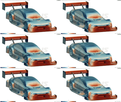
Turbulence involves a wide range of length and time scales. Because resolving every single scale is computationally prohibitive, various models are used to balance accuracy and cost.
Reynolds-Averaged Navier–Stokes (RANS)
RANS is the oldest and most computationally efficient approach. It solves an ensemble version of the governing equations, introducing Reynolds stresses. It can be used for both steady and statistically unsteady flows (URANS). RANS models are often categorized by the number of transport equations they solve, such as the "Zero Equation" Mixing Length model or the "Two Equation" k-ε model.
Large Eddy Simulation (LES)
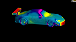
LES filters out the smallest scales of flow and models them using subgrid scale models, while resolving the larger, more energetic scales. It is more accurate than RANS but requires significantly more computational power.
Detached Eddy Simulation (DES)
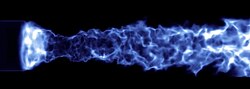
DES is a hybrid approach. It uses RANS near solid boundaries (where turbulent scales are small) and switches to LES in regions where the grid is fine enough to resolve larger eddies. This reduces the computational cost compared to pure LES.
Direct Numerical Simulation (DNS)
DNS is the most accurate method as it resolves the entire range of turbulent length scales without any modeling. However, its cost is proportional to the cube of the Reynolds number (Re³), making it impractical for complex geometries.
Specialized CFD Applications
Two-Phase Flow
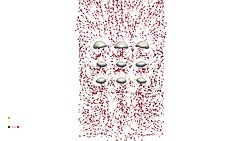
Simulating the interaction between two different phases (e.g., liquid and gas) involves methods like the Volume of Fluid (VOF), level-set, and front tracking. These methods must balance the need for a sharp interface with the requirement for mass conservation.
Biomedical Engineering
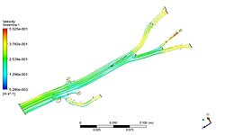
CFD is used to analyze aortic flow by extracting CAD models from MRI or CT scans. By incorporating blood density, viscosity, and systemic pressure, researchers can optimize cardiovascular treatments.
Hardware Acceleration: CPU vs. GPU
Traditionally, CFD has relied on CPUs. However, there is a shift toward GPUs, which feature a larger number of slower processors. Algorithms with high parallelism, such as the Lattice-Boltzmann method, see significant speed-ups on GPU hardware.
Key Facts
- FVM is preferred for combustion and high Reynolds number flows due to its conservation properties and speed.
- DNS is the most accurate turbulence method but is computationally intractable for complex shapes.
- DES acts as a hybrid, switching between RANS and LES to optimize cost and accuracy.
- Vortex Methods are meshfree, making them ideal for acoustic analysis.
- GPU acceleration is most effective for highly parallel algorithms like Lattice-Boltzmann.
| Method | Primary Advantage | Primary Disadvantage | Typical Use Case |
|---|---|---|---|
| Finite Volume (FVM) | Memory efficient, fast | Lower accuracy for smooth problems | General CFD, Combustion |
| Finite Element (FEM) | Stable, handles complex geometry | High memory usage, slower | Structural analysis, smooth fluids |
| Spectral Element | Rapid convergence, high accuracy | Complex mathematical formulation | Academic research, high-precision |
| Vortex Method | Meshfree, no grid smoothing | Requires N-body problem solutions | Incompressible turbulent flows |
Frequently Asked Questions
What is the difference between RANS and LES?
RANS models the effect of all turbulence using time-averaging, making it computationally cheap. LES resolves the large scales of turbulence and only models the smallest scales, providing higher accuracy at a higher computational cost.
Why is DNS rarely used in industrial applications?
DNS resolves every single turbulent scale, meaning the computational cost increases exponentially with the Reynolds number (Re³). This makes it too expensive for the complex geometries found in industry.
What is the purpose of a flux limiter in high-resolution schemes?
Flux limiters are used in high-resolution schemes to prevent spurious oscillations (numerical noise) when capturing sharp changes or shocks in the fluid flow, ensuring the solution remains total variation diminishing.
How does DES improve upon RANS and LES?
Detached Eddy Simulation (DES) combines the strengths of both: it uses RANS for the boundary layers near walls and LES for the separated flow regions, reducing the grid requirements compared to pure LES.
Can CFD be used for medical purposes?
Yes, CFD is used in biomedical engineering to simulate blood flow in the human aorta. By using MRI or CT data to create 3D models, clinicians can analyze cardiovascular health and optimize treatments.